Understanding rainfall statistics

This article presents a step-wise approach to give design practitioners an idea of where figures like the 90th percentile event and concepts like 5 mm retention = 50% annual water balance target = 0.5 runoff coefficient come from. See also drainage time.

The Ontario Ministry of the Environment Conservation and Parks, and other regulatory agencies perform much more rigorous statistical analyses than the example presented, and their resultant stormwater management targets vary accordingly.

Example: City of Barrie, using only years 2015 to 2017

Daily rainfall records from BARRIE LANDFILL weather station were obtained for the years 2015 - 2017, from the Environment Canada historical data record.

The example will only consider rainstorm events, although the records also contain data for 'precipitation'. Precipitation is more useful if snowfall were also of interest to the analyst. (For example, if the analyst wished to calculate annual retention or runoff from a facility.)

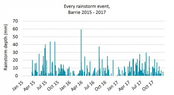
This graph shows the data as a time series:

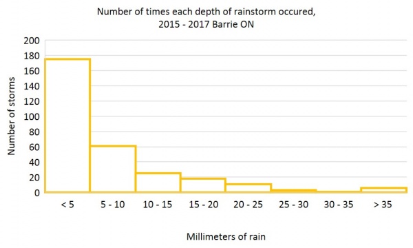
The number of times each depth of storm occured can be counted and grouped like this:

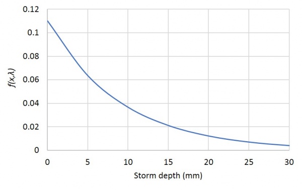
These same data can be fitted to a single equation which would then allow predictions to be made. In this example an exponential distribution function has been selected and an online tool used to find the fitting parameter 'λ'.

$f\left(x,\lambda \right)=\lambda e^{-\lambda x}$

The fitting found λ to be 0.11. When the equation is plotted, the graph looks like this:

But the frequencies of the different rainstorms aren't very easy to understand like this.

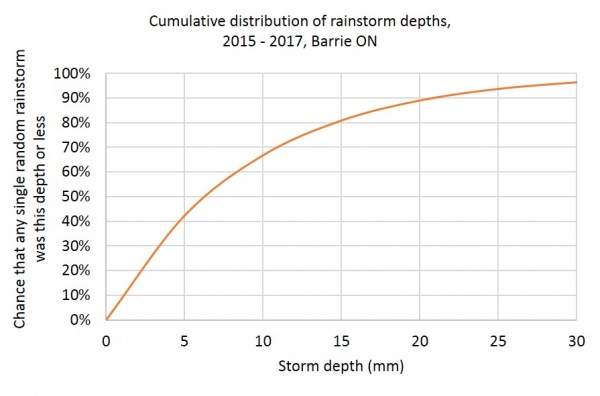
The cumulative distribution function uses the same λ and is a more useful way to read the data.

$F\left(x,\lambda \right)=1-e^{-\lambda x}$

Plotted, it looks like this:

The 90th percentile event is the rainstorm for which 90% of all rainstorms are this depth or less. In this example, using a very limited data set it was found to be 20 mm.

i.e. 90% of all storms ≤ 20 mm.

Storms of ≤ 5 mm represent 40% of the total in this example.

The accounting of inflow and outflow of water in a system according to the components of the hydrologic cycle.

The portion of water precipitated onto a catchment area, which then flows as surface discharge from the catchment area past a specified point.

Water from rain, snow melt, or irrigation that flows over the land surface.

Refers to the conditions in which an organism lives and survives or the conditions in which an organism resides. These conditions can be described as aspects of a “physical”, “social” or an “economic” environment, depending on the perspective perceived by the observer.

Any form of rain or snow.

Any form of rain or snow.